


Table of Contents
Categories
Most Popular


In the part 1 and part 2 of the series, we looked at ways to compare numerical variables and categorical variables. Let’s now look at techniques to compare mixed type of variables i.e. numerical and categorical variables together. Please read this article to visually analyze the relationship between mixed type of variables.
We will work with the same dataset that we worked on in part 2 with the addition of a numerical variable, Revenue.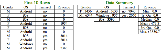
Let us now compare the numerical variable, Revenue with the categorical variables. But, again the techniques learnt in part 1 and part 2 wouldn’t help in this case due to the difference in types of variables involved. If you look at the levels of the categorical variables closely, Gender and Transact has 2 levels whereas OS has 3 levels.
Some of the questions that may arise are?
a) Can we get some insights for Revenue for each of the levels of the categorical variable?
b) Is there a significant difference in Revenue between levels of each categorical variable or are they the same?
Let’s address the above questions in detail:
a) Can we get some insights for Revenue for each of the levels of the categorical variable?
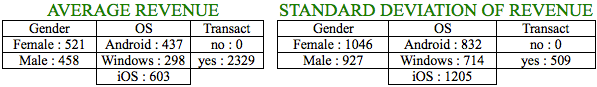
The above tables show the mean and the standard deviation of Revenue for each of the levels in the categorical variables. It is amply clear that the above revenue statistics for users across different levels in the categorical variables are different.
Few Insights from Average Revenue
- iOS users are highly valuable compared to Windows users since the average spend of iOS users is more than double of Windows users and 38% higher than Android users.
- Female users on an average have spent 13.7% more than Male users.
Similarly, we can draw out insights based on standard deviation and extend the analysis further based on other summary statistics like median, quantiles, etc.
b) Is there a difference in Revenue between levels of each categorical variable or are they same?
It is amply clear from points discussed in (a) that there is a difference. But, the important question is there a statistical difference, based on which one could take appropriate actions?
Revenue & Gender
Let’s begin with comparing Revenue and Gender, which has 2 levels. We will use the mean/average Revenue of Male and Female users to check whether the Revenue is impacted by Gender of the person i.e. is the higher average spend of Female users over Male users statistically significant? We will use Hypothesis Testing discussed in part 2 to answer the same. Please refer part 2 to understand some of the concepts discussed hereinafter.
H0: There is no difference in the means (Mean Revenue of Male Users = Mean Revenue of Female Users)
H1: There is a difference in means (Mean Revenue of Male Users ≠ Mean Revenue of Female Users)
We will use a statistical test known as t-test to test our hypothesis. Similar to chi-square test, we will calculate the t-statistic, degrees of freedom and get the p-value to compare it against the assumed alpha to conclude whether we can accept or reject the null hypothesis.
t-statistic = 4.0026
p-value for the t-statistic at 1 degree of freedom = 0.1559
Since p-value is greater than the assumed alpha of 0.05, we fail to reject the null hypothesis and conclude that there is no difference in Mean Revenue of Male and Female Users i.e. Gender of the user does not impact the Revenue of the app.
Revenue & OS
Can we use t-test to compare the mean Revenue across levels of OS? OS has 3 levels. In t-tests, you compare 2 means at a time. So, you will have to compare 3 combinations of means for OS since it has 3 levels. For those 3 combinations, you will need to test 3 hypotheses as enlisted below:
i) H0: Mean Revenue of Android users = Mean Revenue of iOS users
ii) H0: Mean Revenue of Android users = Mean Revenue of Windows users
iii) Ho: Mean Revenue of iOS users = Mean Revenue of Windows users
Each of the tests has an assumed alpha of say 5%. So essentially, the 5% chance of a wrong prediction for each test gets accumulated resulting in approximately 15% chance of error (14.3%* to be precise). The error rate compounds for multiple t-tests.
*Combined alpha = 1 – (0.95 * 0.95 * 0.95) = 14.3%
But, we didn’t want the alpha to be greater than 5%. Hence, multiple t-tests won’t work in this case. In cases where we have to compare more than 2 means, ANOVA is a better option.
Analysis of Variance (ANOVA)
In order to understand if the levels in the categorical variables affect Revenue, you need to test the following hypothesis:

In simple terms, before identifying the categorical level for which the mean Revenue is different, you ideally would want to first know if there exists a difference in at least one of the means of the categorical levels.
Let’s understand the above formula with help of an example:
Suppose you need to analyze the marks of students in 5 divisions of a class. More specifically, you need to know whether the average marks of at least one division significantly differs from the average marks of the entire class. ANOVA tries to answer it by breaking down the source of variation.
Total Variation = Variance Between the means + Variance Within the means
The numerator, in the ANOVA formula, calculates the variation in average marks of each division from the average marks of the entire class. The denominator calculates the variation of the marks of each student in each division from the average marks for that division. The ratio of the numerator to denominator helps us to conclude if the average marks of at least one of the divisions is significantly different from the average marks of the entire class. The ratio, which is further and further away from 1, implies that such difference could be statistically significant.
We used the chi-square statistic in part 2 to ascertain the p-value. Here, we will use the F statistic to ascertain p-value for the hypothesis test concerning OS and Revenue.
F-statistic = 50.22
We need to check the F-statistic against the F distribution table or use statistical software to arrive at the p value.
The p-value for the ANOVA between OS and Revenue yielded a value < 2e-16 or almost zero. Hence, we can reject the null hypothesis and conclude that the type of OS has an effect on Revenue from the user. We can dig deeper and use statistical tests like Tukey’s HSD to understand which particular level(s) of the categorical variable has statistically different mean.
What we have looked above is a one-way ANOVA where we analyzed the relationship between a numerical and categorical variable. We can extend this to analyze a numerical variable and more than 1 categorical variable at the same time.
Closing Thoughts
In this series, we have introduced the below techniques to compare variables and make better sense of data.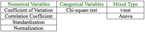
Comparing variables, which differ in scale, type, etc. is not an option but a need that could bring out patterns and valuable insights in data. Based on the type of variables, the context and the objective of such comparison, it is prudent to judiciously use the right technique to compare them, else it may lead to poor results.
Jacob Joseph 
Heads Data Science.Expert in AI, Data & Analytics and awarded 40 under 40 Data Scientists in India.
Free Customer Engagement Guides
Join our newsletter for actionable tips and proven strategies to grow your business and engage your customers.