


Table of Contents
Categories
Most Popular


In the previous article, we looked at some of the ways to compare different numerical variables. In this article, we shall look at techniques to compare categorical variables with the help of an example.
Assume you have been given a dataset totaling 10,000 rows containing user information on Operating System, Gender and whether the user has transacted over a particular period.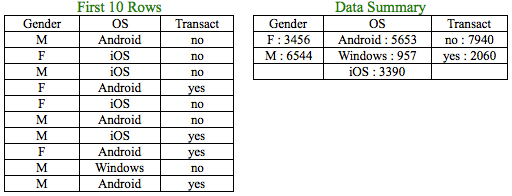
All the variables mentioned above are categorical variables. It seems 35% of the users are Female and 65% Male. Female Android users constitute 25% and Male Android users constitute 75% of the Android users. If there is no association between Gender and OS, you will expect that the percentage composition of Female Android and Male Android users (25% & 75%) will be similar to that of the percentage composition between Female and Male users (35% and 65%). The same holds true for Windows and iOS users. But, is there a way to conclude if the observed difference is big enough to concur that the percentage composition indeed is not similar? In short, we are trying to ask the question ‘Is there an association between the categorical variables – Gender and OS?’.
Since we are dealing with categorical variables, we cannot use the techniques like coefficient of variation or correlation coefficient used to analyze numerical variables.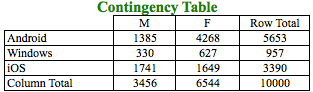
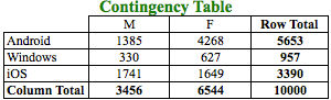
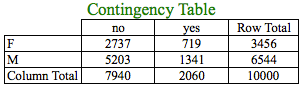
In order to compare categorical variables, we have to work with frequency of levels/attributes of such variables. From the above table, we know that the frequency of ‘Android’ in OS is 5653 users of which Male users are 1385 and Female users are 4268 as can be seen in the first row of the table. We need to use this frequency to compare the categorical variables. The above table is a Contingency table where we are analyzing 2 categorical variables. A contingency table is essentially a display format used to analyze and record the relationship between two or more categorical variables. Let’s further analyze the contingency table: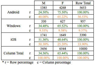
From the above table, it seems that the break-up of Gender is different across Operating System. For example:
- Android users constitute 56.53% of the total users. But, if we segregate the users based on Gender, we get different percentages for Males and Females on Android.
- Male Android users constitute 40.08% of the Male users whereas Female Android users constitute 65.22% of the Female users.
The question that may arise is why there is a difference in the frequency percentages when we look at levels in a single category compared to the combination of levels of more than 1 categorical variable. Is there an association between the Gender and OS resulting in the difference? Is this deviation in percentages statistically significant to conclude the presence of some association?
Statistical significance
We often come across the term ‘statistical significance’ or ‘random chance’. But what does it mean intuitively?
Imagine you are tossing 2 coins, A and B 10 times. Coin ‘A’ landed heads 3 times whereas Coin ‘B’ landed heads 5 times. Does it mean that Coin ‘A’ is an unfair coin where chances of landing tails are more than heads? You know intuitively that the difference could have occurred simply due to luck or by chance. But, what if you have tossed the coins 1000 times and Coin ‘A’ landed heads 100 times whereas Coin ‘B’ landed heads 550 times? Would you still attribute this difference to chance or some other underlying factors such as the shape of the coins? We can answer this difference with the help of statistical tests.
Coming back to our discussion on our example of User data, we will attempt to answer the difference seen in the contingency table with the help of Hypothesis testing.
Hypothesis testing
Claim 1: Gender is independent of Operating System (No Association)
Claim 2: Gender is not independent of Operating System (Association)
The above 2 claims/statements are essentially what we test in hypothesis testing. We deal with hypothesis on a daily basis. We might have hypothesis on political issues, social issues, financial issues, etc. For example, we might have a hypothesis on whether it will rain today?
In any hypothesis, you will have a default or null hypothesis referred to as H0 (Claim 1), which is your default belief and an alternate hypothesis referred to as H1 (Claim 2), which is against your default belief. The null hypothesis is the statement being tested. Usually the null hypothesis is a statement of “no effect” or “no difference”.
So, in our example, we would expect the percentage composition of Gender to be the same for Android, Windows and iOS users (Null Hypothesis). The Alternate Hypothesis is that we don’t expect it to be the same. Here, the word ‘same’ does not imply that the percentage composition has to be exactly equal but it means that there is no statistical difference. We run some appropriate statistical tests to determine it i.e. whether to accept or reject the null hypothesis.
But, prior to that, we need to understand 3 statistical concepts, (i) p-value (ii) chi-square statistic (iii) degrees of freedom
i) What is p-value ?
Assuming you have a hypothesis (in the above case, Gender and OS are independent of each other), the p-value helps you evaluate if the null hypothesis is true. Statistical test use p-value to determine whether to accept or reject the null hypothesis. It measures how compatible your data is with your null hypothesis or the chance that you are willing to take in being wrong. For example, a p value of 0.05 and 0.1 means you are willing to let 5% and 10% of your predictions be wrong respectively.
In other words, p-value is the probability of observing the effect by chance in your data, assuming the null hypothesis is true. So, lower the p-value, lower the probability of observing the effect by chance or at random, and higher the probability of rejecting your default or null hypothesis. In practice, depending on your area of study, generally you have cut-off levels like 1% and 5% for p-values below which you could conclude that the effect is not random or by chance and the null hypothesis could be rejected.
ii) What is Chi-square statistic ?
Before understanding chi-square statistic, let’s understand the concept of observed and expected frequencies.
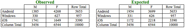
Observed frequencies are the actual frequencies as seen in the data and shown in the contingency table above as ‘Observed’. This is the same contingency table, we had introduced earlier. Expected frequencies are frequencies we could expect if there was absolutely no association and shown in the contingency table above as ‘Expected’.
How did we calculate the expected frequency? Expected frequency is calculated from the observed or actual frequencies.

Let’s analyze the expected frequencies further:
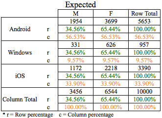
In the above table, the row and column percentages are quite similar and there doesn’t seem to be a difference in percentages due to the influence of Gender on OS or vice-versa.
Chi-square test is a statistical test commonly used to compare observed data with the data we would expect to obtain according to a specific hypothesis. In our example, we would have expected 1954 of 5653 Android users to be Male but actual or observed were 1385. So is this deviation of 569 users statistically significant? Were the deviations (differences between observed and expected) the result of chance, or were they due to other factors? The chi-square test helps us answers this by calculating the chi-square statistic.
That is, chi-square statistic is the sum of the squared difference between observed and the expected data, divided by the expected data in all possible categories.
iii) What is Degrees of Freedom ?
The degrees of freedom is the number of values in a calculation that we can vary. Let’s understand degrees of freedom with the help of an example.
Example 1:
Suppose you know that the mean for a data with 10 observations is 25 and that variable has many such sets of 10 observations. So, for a new set of 10 observations, we have the freedom to set the value of 9 observations i.e. you can have the freedom to select any 9 values. But, you won’t have the freedom to set the value for the 10th observation. This is because the mean of the data has to be equal to 25. So the value of the 10th observation has to be equal to (25 * 10 – sum of the values of 9 observations). Hence, the degrees of freedom in this case is 9.
Example 2:
In order to run a chi-square test on the contingency table, the row total and the column total is like the mean and the other cells in the contingency table are like the observations in the Example 1. In the above contingency table, we can only freely select 2 values so that the row and column totals are not changed. Hence degrees of freedom is 2. The formula to calculate it for a contingency table with 2 categorical variables is (r – 1) * (c – 1), which for our case is (3 – 1) * (2 – 1) = 2
Steps to calculate p-value
In order to accept or reject the Null Hypothesis, we need to calculate the p-value. p-value is calculated in the following 3 steps:
Step 1) Calculate Chi-square statistic
Step 2) Calculate the degrees of freedom
Step 3) Find the p-value corresponding to chi-square statistic with corresponding degrees of freedom in the chi-square distribution table.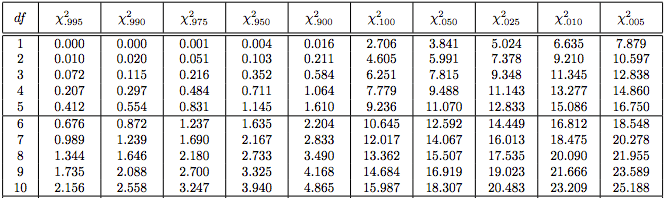
The above table is an excerpt of a chi-square distribution table. The first column contains degrees of freedom. The cells of each row give the critical value of chi-square for a given p-value (column heading) and a given number of degrees of freedom. For a given degrees of freedom, higher the chi-square statistic (cell value), lower the p-value.
OS & Gender
In our example, the Chi-square statistic (χ2) for OS and Gender using the chi-square statistic formula = 675.86.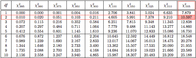
In the chi-square distribution table, χ20.005 statistic is 10.597 at 2 degrees of freedom. Hence, the p-value has to be less than 0.005. This can be easily solved using a computer rather than manually.
p-value or P (χ2 > 675.86) at 2 degrees of freedom < 2.2e-16 or almost zero.
We have to compare this p-value with an assumed cut-off level of 5% or 1% known as alpha or significance level. The assumed alpha value helps to conclude if the statistic is observed by chance or by any other factor. The p-value calculated is less than the assumed alpha. Hence, we can say that based on the evidence, we fail to accept or reject the Null Hypothesis and conclude that Gender and OS are not independent.
Gender & Transact
χ2 = 0.11647
P (χ2 > 675.86) at 1 degree of freedom = 0.7329
Since p-value is greater than the alpha value of 0.05, we fail to reject the Null Hypothesis and conclude that Gender and Transact are independent.
OS & Transact

χ2 = 24.581
P (χ2 > 24.581) at 2 degrees of freedom = 4.595e-06 or almost zero.
Since p-value is less than the alpha value of 0.05, we reject the Null Hypothesis and conclude that OS and Transact are not independent.
Closing Thoughts
To sum up, we have been able to compare 2 categorical variables with the help of contingency table and chi-square test. The same concept can be extended to compare more than 2 categorical variables together. The next article will deal with ways to compare mixed type of variables i.e. when we have to deal with numerical and categorical together.
Jacob Joseph 
Heads Data Science.Expert in AI, Data & Analytics and awarded 40 under 40 Data Scientists in India.
Free Customer Engagement Guides
Join our newsletter for actionable tips and proven strategies to grow your business and engage your customers.