


Table of Contents
Categories
Most Popular


Neural networks, as the name suggests, involves a relationship between the nervous system and networks. It’s a relationship loosely modeled on how the human brain functions.
And it’s used in many modern applications, including: driverless cars, object classification and detection, personalized recommendations, language translation, image tagging, and much more.
What are Neural Networks?
A neural network is either a biological neural network, made up of real biological neurons, or an artificial neural network, designed to recognize patterns and solve business problems.
Neural Networks: How They Mimic the Brain
Artificial neural networks try to mimic the biological neural network in the human brain.
Nature has inspired millions of innovations – everything from birds inspiring airplanes, burdocks inspiring velcro, to whales inspiring wind turbines to go faster. In the same way, the human brain has inspired the creation of neural networks.
A typical brain contains close to 100 billion miniscule cells called neurons. Each neuron is made up of a cell body with a number of connections coming off it: numerous dendrites (the cell’s inputs—carrying information toward the cell body) and a single axon (the cell’s output—carrying information away).
Dendrites extend from the neuron cell body and receive messages from other neurons. When neurons receive or send messages, they transmit electrical impulses along their axons that aid in carrying out functions such as storing memories, controlling muscles, and more.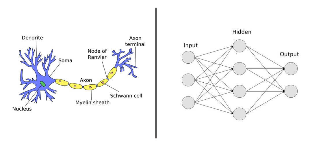
There are areas, however, where the simplified model of the artificial neural network does not quite mimic the brain exactly. For example, it can’t mimic the creation or destruction of connections (dendrites or axons) between neurons, and it ignores signal timing.
Still, artificial neural networks are quite effective considering how they’re used in many applications, and have become smarter over time.
How Do Neural Networks Work, Exactly?
Let’s try to understand how these neural networks function by looking at their inner workings. (Warning: there will be mathematics involved.)
Have a look at the following table:
| x | y |
|---|---|
| 0 | 0 |
| 1 | 4 |
| 2 | 8 |
| 3 | 12 |
| 4 | 16 |
Its a pretty dumb example. One can clearly make out that y = 4 * x. But here’s how a neural network would try to derive the relationship between y and x.
Step1: Random Guess
We have to start somewhere. Let’s randomly guess the desired multiplier is 2.
The relationship will now look like y = 2 * x
Step 2: Forward Propagation
Here we are propagating the calculation forward from the input —> output. So now the table would look like this:
| x | Predicted y’ |
|---|---|
| 0 | 0 |
| 1 | 2 |
| 2 | 4 |
| 3 | 6 |
| 4 | 8 |
Step 3: Error
Let’s compare the prediction versus the actual.
| x | Actual y | Predicted y’ | Squared error(y-y’)2 |
|---|---|---|---|
| 0 | 0 | 0 | 0 |
| 1 | 4 | 2 | 4 |
| 2 | 8 | 4 | 16 |
| 3 | 12 | 6 | 36 |
| 4 | 16 | 8 | 64 |
| TOTAL | 120 | ||
We calculate the error as the square of deviation of the actual from the predicted y’. This way we penalize the error irrespective of the direction of error.
Step 4: Minimize Error
The next logical step is to minimize the error. We randomly initialized 2 as the multiplier. Based on that, the error was 120. We can try with many other values say ranging from -100 to 100.
Since we know the real value (4), we will end up with the correct value pretty quickly. But, in practice, when you deal with a lot more variables (here there is only one: x) and with more complex relationships, trying out different random values for x is not scalable, and definitely not an efficient use of computing resources.
Derivatives
A popular way to solve this problem is with the help of differentiation or derivatives. Basically, derivatives are the rate of change of a function with respect to one of its variables. In our example, it is the rate of change in the error or loss function with respect to x.
To observe the effect of change, let’s change the multiplier or weight or the parameter from 2 to 2.0001 i.e. increase it by 0.0001 and also decrease it by the same amount. In practice, this increase is even smaller.
Let’s observe the impact:
| x | Actual y | Weight = 2 | Squared error @ 2 | Weight = 2.0001 | Squared error @ 2.0001 | Weight = 1.9999 | Squared error @ 1.9999 |
|---|---|---|---|---|---|---|---|
| 0 | 0 | 0 | 0 | 0 | 0 | 0 | 0 |
| 1 | 4 | 2 | 2 | 2.0001 | 3.99 | 1.9999 | 4.0004 |
| 2 | 8 | 4 | 16 | 4.0002 | 15.99 | 3.9998 | 16.0016 |
| 3 | 12 | 6 | 36 | 6.0003 | 35.99 | 5.9997 | 36.0036 |
| 4 | 16 | 8 | 64 | 8.0004 | 63.99 | 7.9996 | 64.006 |
| 4 | 16 | 8 | 64 | 8.0004 | 63.99 | 7.9996 | 64.006 |
| TOTAL | 120 | 119.988 | 120.012 | ||||
With increase in weight by 0.0001, the loss decreased by 0.012 and with a decrease in weight, the loss increased by 0.012. For a 0.0001 increase in weight, the loss decreased by 120 times (0.012 / 0.0001).
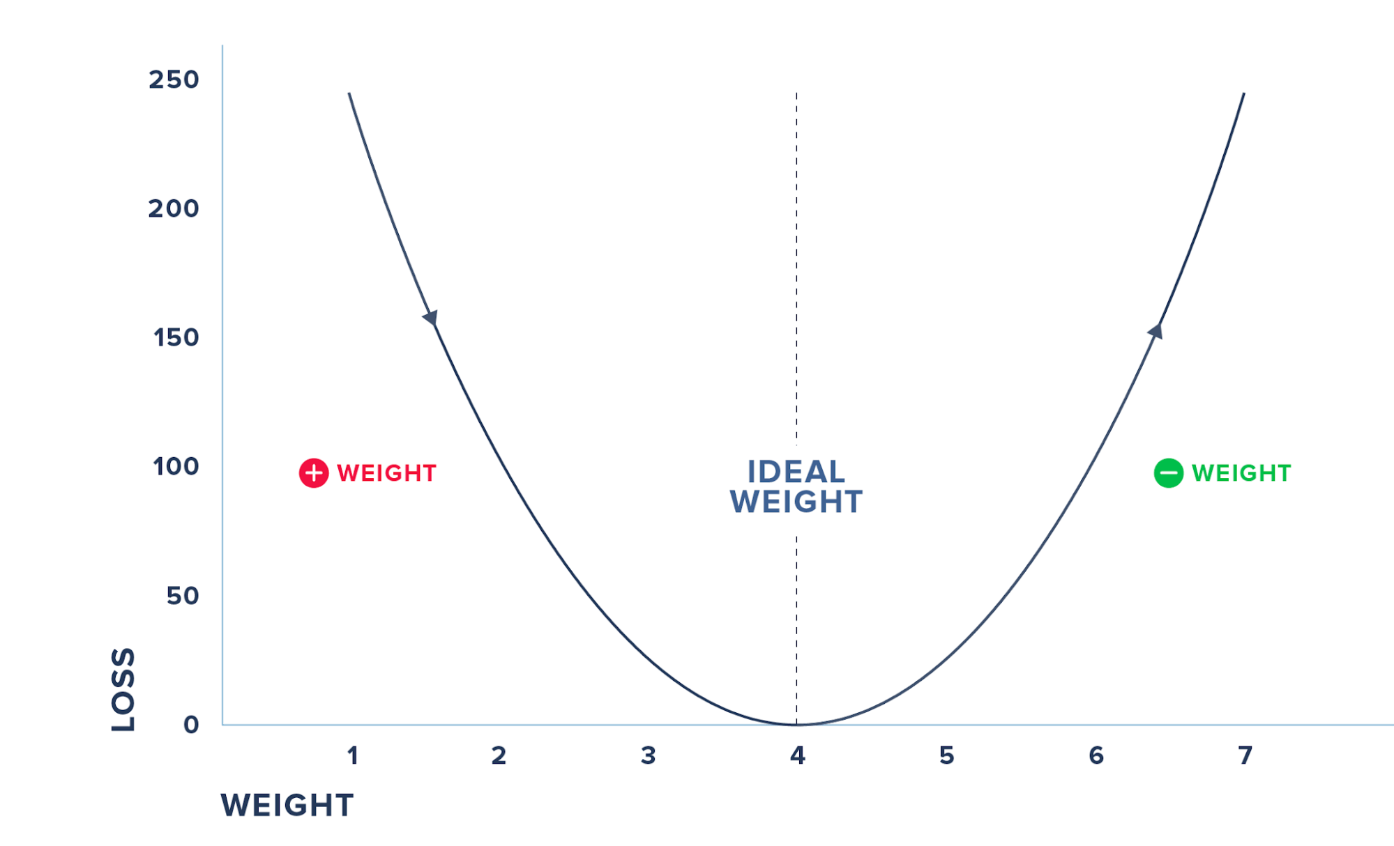
So how much should we increase the weight to reduce the loss? If we take some different arbitrary number such as 7, the loss increases to 270. So we know now that the weight should be somewhere between 2 and 7.
Findings:
- If we decrease the weight from 2, the loss increases
- If we increase the weight from 2, the loss decreases up to a point and then it increases as loss is high at weight = 7
We cannot do this iterative process of randomly checking for various weights and arriving at the magical parameter. Moreover, in practice, you will have to deal with many input variables and not just one. Hence we use derivatives where we check the effect on loss for a small change in the input.
The above figure summarizes the steps where we check for the derivative and increase the weights, if the loss decreases and vice-versa before we hit the weight where the loss reaches 0. We do this iteratively and update the weights and the loss till we minimize the loss to 0.
The process by which we calculate the derivatives needed in the calculation of weights is called back propagation.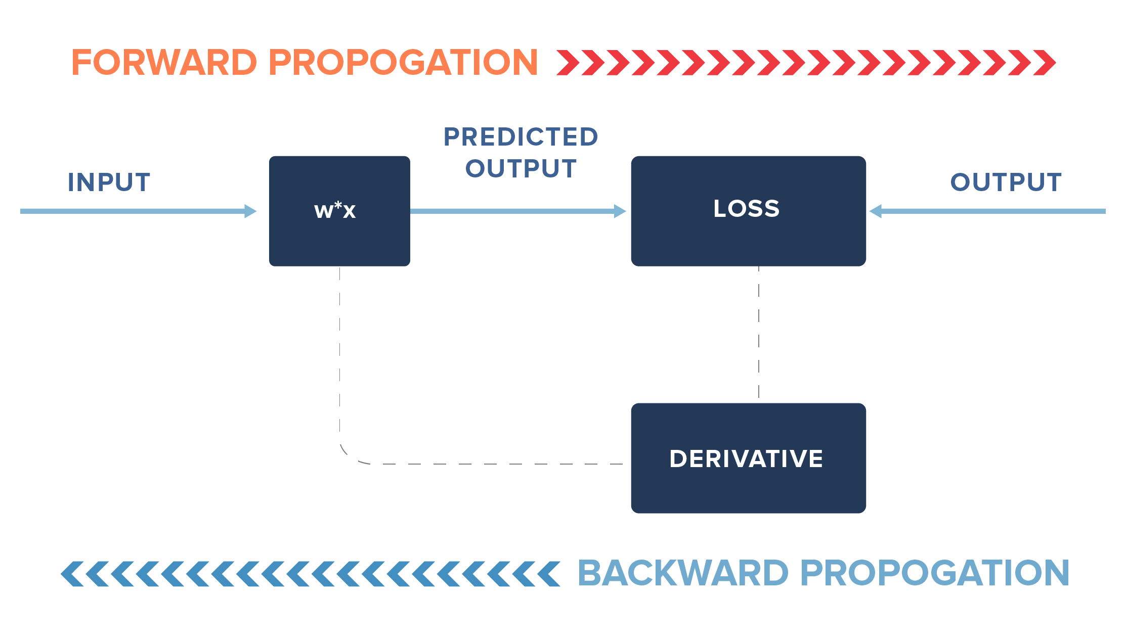
In practice, we may not update our weights fully but only by a fraction of the new learned change in weights (i.e. instead of 0.0001, we may update it by a fraction of 0.0001). Additionally, we may stop earlier than the loss reaches 0, say for example, we may stop if the loss reaches 0.000001.
But wait, this is not how we generally imagine or view neural networks. It looks more like this: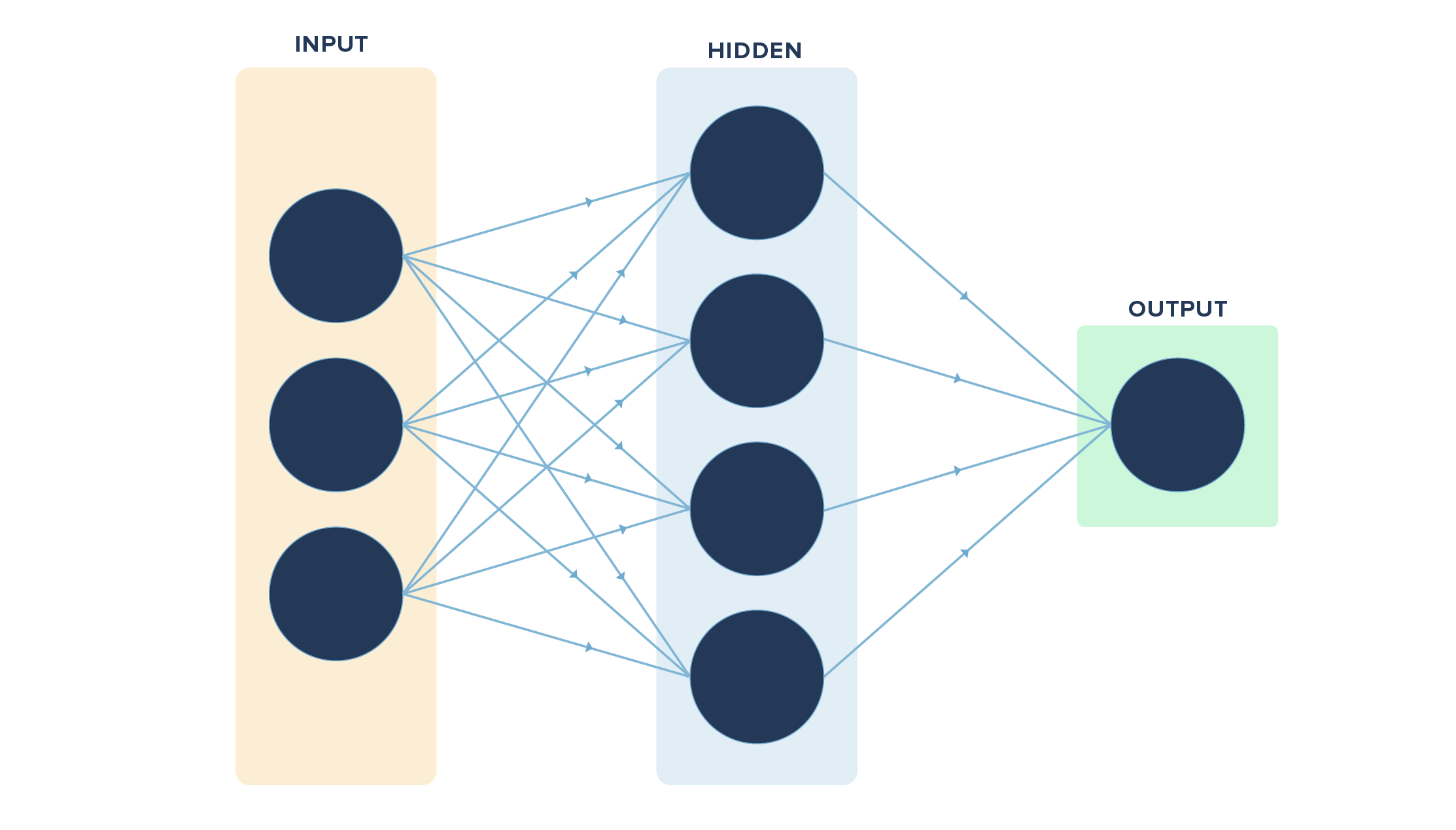
So what’s so different from our example?
The key differences are in the number of variables used (multiple vs. one in our case), the layers in between the input and the final output (hidden layers, which are missing in our example) and the output (multiple vs. one in our case).
If we convert our example visually, it will look like this: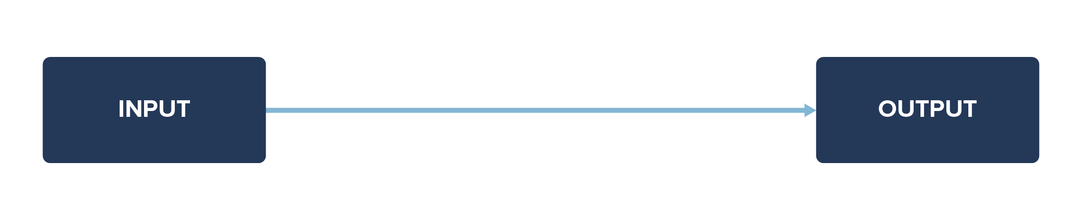
We had a simple task/function in hand to learn. What if we had a complex function to learn with many input variables ranging from x1, x2, ……, xn (n variables)? It may not be possible to learn everything directly. So we may have layers between the input and output layers to make it easier for the neural net to learn the function.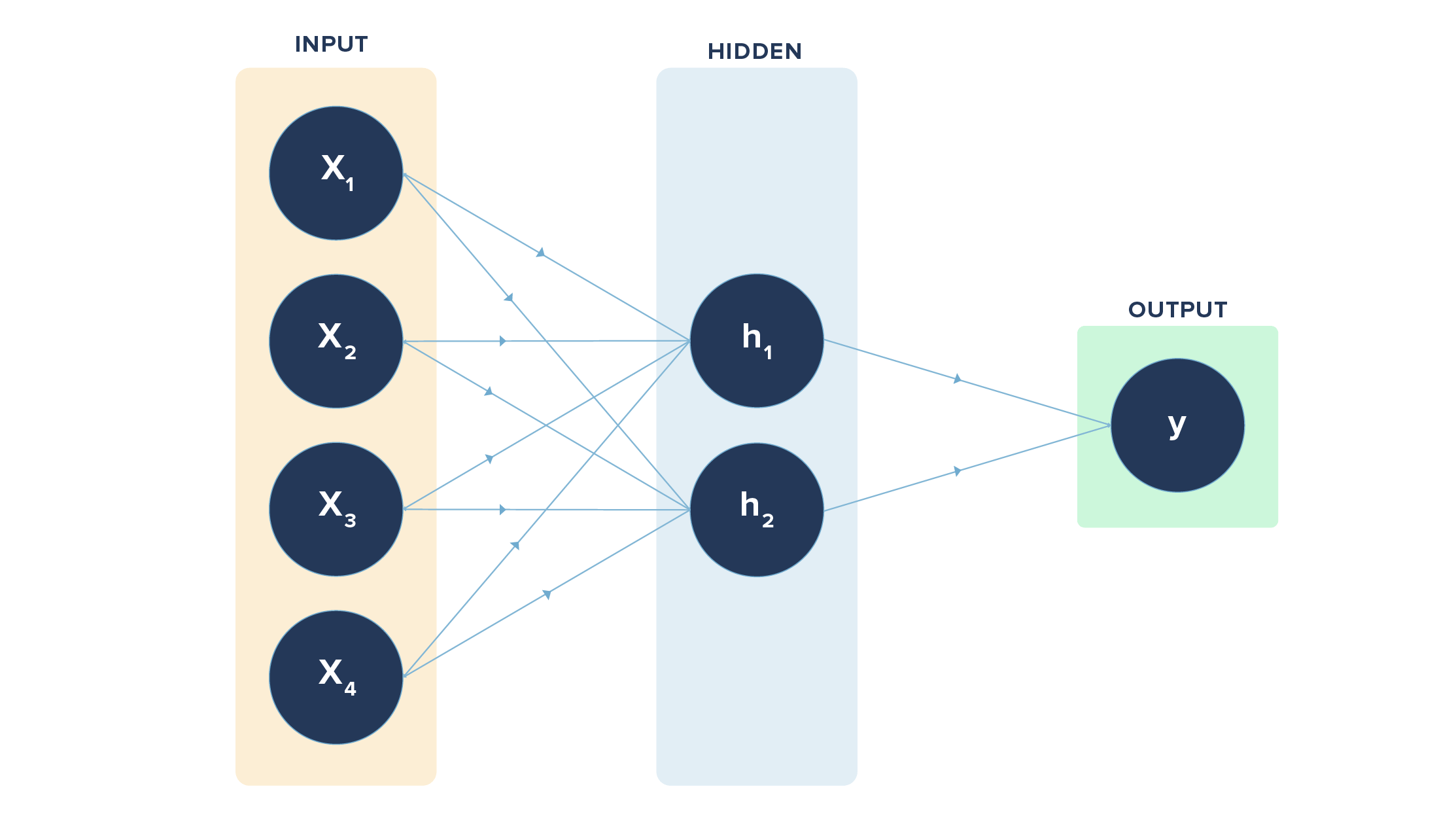
In the above diagram, we have 4 inputs or nodes in the input layer, 2 nodes in the hidden layer, and 1 node in the output layer. The lines indicate the connection each node has with the node in the layer following it. The connections are through the weights involved, which are learned via forward and back propagation.
h1 = x1 * w1 + x2 * w1 + x3 * w1 + x4 * w1
h2 = x1 * w2 + x2 * w2 + x3 * w2 + x4 * w2
Here, “w” refers to weights connecting input layer to hidden layer. Likewise, we have a set of weights from hidden layer to output layer.
The earlier case had just one of the input nodes and one output node with the connection. In case we are tasked with classifying items such as digits from 0 to 9 (multi-class output), we will have 10 nodes (each digit represented by one node) in the output layer instead of one. Likewise, we can have multiple hidden layers too.
How’s That for a Primer?
This blog post is intended to help the reader understand neural networks from the ground up and make it easier to comprehend its inner workings. This is just the beginning of your journey into the infinite possibilities with neural networks.
CleverTap’s data science engine uses neural networks to power its recommendation system.
In forthcoming posts, we will discuss how we enable the recommender engine of CleverTap with neural networks and orchestrate the entire recommender engine pipeline.

See how today’s top brands use CleverTap to drive long-term growth and retention
Jacob Joseph 
Heads Data Science.Expert in AI, Data & Analytics and awarded 40 under 40 Data Scientists in India.
Free Customer Engagement Guides
Join our newsletter for actionable tips and proven strategies to grow your business and engage your customers.