


Table of Contents
Categories
Most Popular


Why do we need experiments?
Experiments play an important role to test theories and provide the basis for scientific knowledge. Similarly, experiments are an important tool for product and marketing analytics. Product experts and growth marketers are looking for ways to increase conversions and engagement, reduce churn, and so on. An essential tool with the experimentation framework are A/B tests.
What are A/B tests?
A/B tests are extremely powerful and useful tools to test content. A/B testing is a method of comparing two versions of a web page or app to determine which one performs better. You can extend it to multivariate testing, where more than two variants can be compared.
How does one design a good A/B test?
A/B tests involves
- Testing different types of content
- Selecting the number of users being tested
- Time period of testing
In order to conduct a proper A/B, you need to:
- Identify the ideal variant size
- Maintain a disciplined approach on measurement
Let’s say you are tasked with improving the conversions on your landing page that currently stands at a 2% conversion rate. You have another variation of the landing page in production that you would like to compare to the live one.
Let’s understand some basics of statistics to achieve our goal.
Basic Understanding of few statistical concepts
While comparing both variants, you wouldn’t want a scenario where a variant showed a 20% lift in conversions during the experiment. However, the same variant delivered lower than or no lift compared to the default version in production most of the time. In other words, the outperformance during experiment could be by chance or random.
Here’s how you minimize this risk:
- Hypothesis Testing
Hypothesis testing refers to the formal procedures used by statisticians to accept or reject their predicted outcome of the test.
Types of hypotheses:- Null Hypothesis – Assumes the observation occurred due to a chance or is random. In case of A/B testing, we stick to the default version by saying that there is no difference in the variants.
- Alternative Hypothesis – When sample observations are influenced by some non-random cause or are a result of real-effect. Here, we would say there indeed is a difference.
- Level of Significance
We cannot avoid risk or significance. We can only minimize it.
Level of significance refers to the degree we accept or reject the null hypothesis. For example, if you assume there is no underlying difference between the two samples/variants, how often will you see a difference by chance? That percentage chance is the significance level. - Types of Risk
There are two types of risk to consider :- False Positive Risk
Popularly known as Type I risk in statistics and False Positive risk in engineering, this is the act of falsely rejecting the null hypothesis when it is true.
In case of A/B testing, you concluded that the challenger variant was better than the default version. In reality, there was no difference. - False Negative Risk
Popularly known as Type II risk in statistics and False Negative risk in engineering, this is the act of failing to reject the Null Hypothesis when it is false.
In case of A/B testing, you concluded that the challenger version wasn’t better than the default one (lack of evidence to reject the null hypothesis). In reality, the challenger variant was better.
- False Positive Risk
We have some preconceptions about the expected lift, beyond which we will accept the challenger. For a 2% default rate and a lift of 20%, the minimum detectable effect is 0.4%.
What are the chances of observing a 0.4% increase in conversion rates when there is no increase in the conversion rate? If the chance or probability is small enough, say less than 5%, we could say that the observed result is probably due to an actual effect.
It is a common practice to set the Type I risk to 5%. It means that in 5% of the times, we will incorrectly say that there is an effect although it was most likely random chance. 95% of the time, we correctly assume the observed effect was just noise and there isn’t an actual effect.
But what about Type II error?
In our example, say we observed either of the following:
- The lift is 15%
- The conversion is 2.3%
- The difference between the two variants is 0.3%.
Because we needed a lift of at least 20%, we should retain the default version.
What is the risk of retaining the default version? The conversion rate of the challenger version may actually be higher and the lower conversion rate was due to chance. Type II error helps us quantify that.
For example, assume that we ran an experiment with 10,000 users for the incumbent variant and the challenger. We need a lift of at least 20% or 2.4% conversion rate (minimum detectable effect) to make the selection of the challenger worthwhile. The challenger variant scored a conversion rate of 2.45% or 22.5% lift, which is clearly above 20%.
Should we reject the incumbent and choose the challenger? What are the risks associated with it? We know that we had assumed the Type I risk at 5%.
At 5%, the Critical value for the lift is 27% or the conversion rate is 2.54%.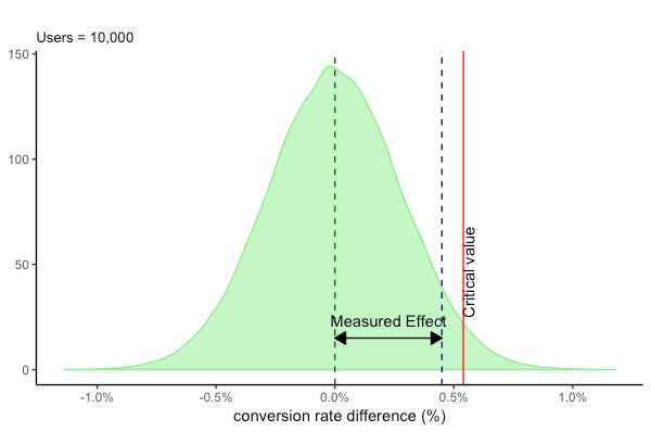
From the figure above, we can infer that for a 5% Type I error, the lift generated isn’t above the critical value.
Is the above analysis enough to reject the challenger variant? What if the observation is random and in reality, challenger conversion rates are beyond 2.54%. For that, we need to look at the distribution of the lift (detectable effects) created by the challenger.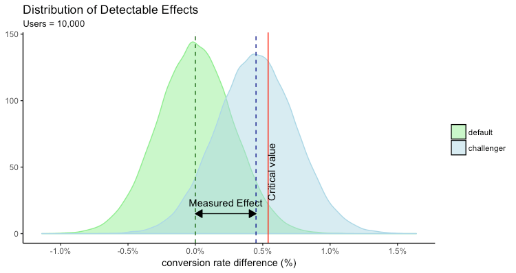
From the above figure, it’s clear that less than half of the possible detectable effects are larger than the critical value (0.54%) shown by the region to the right of the red vertical line. The region to the left is the Type II error, which is larger than 50%. Not a desirable scenario indeed!
How do we reduce the type error in the above scenario? We observe the impact of running the test on higher number of users on the Type II error.
At 50,000 users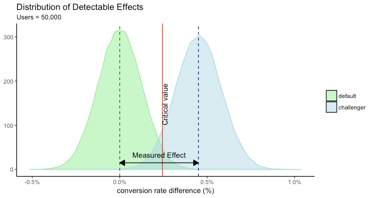
At 100,000 users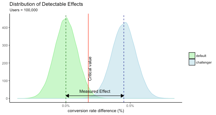
The increase in the sample size had a positive effect on both the Type I and Type II error. Now it is much easier to make conclusion on the tests.
From the statistical concepts discussed above, we know that sample sizes play an important role in determining the strength of such tests. Below is the table of sample sizes at various levels of conversion rates at 5% Type I risk, 20% Type II risk, and minimal detectable difference of 10%
| Conversion Rate | Sample Size per variant |
|---|---|
| 1% | 157,697 |
| 2% | 78,039 |
| 3% | 51,486 |
| 4% | 38,210 |
| 5% | 30,244 |
| 6% | 24,934 |
http://www.evanmiller.org/ab-testing/sample-size.html
Reality Check
We seem to have all the statistical tools to help us create statistically sound A/B tests. However, A/B tests suffer from 3 major problems in practice:
- Sample Size
Unless you have millions of users, it’s very difficult to run A/B tests on a fraction of users.
For example, if the idea was to run a test on 5% of users then you can allocate only 2.5% of the users to each sample. If the required statistically significant sample size is 100,000 then the user base must be at least 4 million. This user base may not be available for small to mid-sized apps. - Peeping
Even if you create the variants with a statistically significant sample size, you might be guilty of peeping into results at regular intervals and get spurious results.
For example, the 2% conversion discussed earlier was for a conversion time over two weeks. If you looked too soon you are bound to get statistically significant results in between. There is a high likelihood that if you had waited for two weeks, the results of the challenger was similar or worse than the default. There are numerous instances when enthusiastic users have stopped the experiment midway to declare a variant as winner.
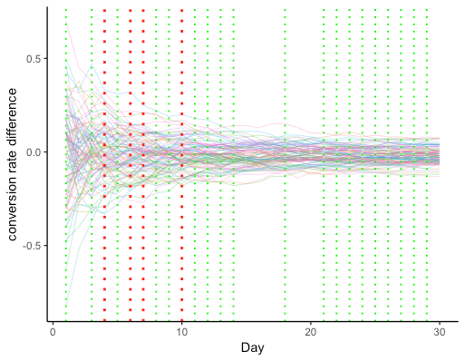
The above figure plots the conversion rate difference between the default variant and the challenger variant conversion on a daily basis for 100 experiments. Both variants have the same overall conversion rate of 2%, if we take the entire duration of 30 days. We ran an A/A test rather than an A/B test here. Both variants are the same.
We assume a significance level of 5% or expect that less than 5 out of 100 experiments in the null hypothesis were wrongly rejected. So ideally out of 100 tests, we expect only up to 5 tests are significant, or in other words, we wrongly reject the null hypothesis up to 5 times out of 100.
The green intercept highlights the days on which the statistical significance was at a 5% level for experiments between 6-9 of the 100 experiments.
The red intercept highlights the days on which 10, or more than 10, experiments had a statistical significance at the 5% level. So clearly, peeping is subject to a lot of risks, especially in the initial days of the experiment.
In an era where experiments, queries, and reports can be run in real time, it is very difficult as a marketer or product expert to design experiments scientifically and adhere to the rules. - Multiple Variants
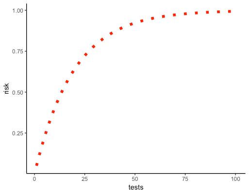
The problem is magnified when you test for multiple variants. The more tests you take, the higher the probability that you obtain at least one false significant result (you reject the true hypothesis).
For example, in addition to the default version A and a challenger B, assume you want to test another variant C. So you end up comparing A with B and A with C. The higher number of tests you run, the greater the probability of type I error. In this case, the error or risk increases to ~10% (1 – (1 – 0.05)2) instead of assumed 5% risk.
The above graph illustrates the increase in error compared to the assumed 5% error rate.
Of course there are some corrections to the multiple testing problems like Bonferroni or Hochberg but they require more statistical knowledge. Additionally, there is an added dilemma of choosing the method best suited to make such corrections. Some are more conservative while others are less conservative.
What is the solution?
To be agile, one has to find a balance between accuracy and speed. In the next post, we will talk about two techniques which give you the flexibility to conclude your tests faster and for lower sample size:
- Sequential AB tests
- Bayesian AB Tests
Jacob Joseph 
Heads Data Science.Expert in AI, Data & Analytics and awarded 40 under 40 Data Scientists in India.
Free Customer Engagement Guides
Join our newsletter for actionable tips and proven strategies to grow your business and engage your customers.