


Table of Contents
Categories
Most Popular


Why would you want to convert a numerical variable into categorical one? Depending on the situation, it can lead to a better interpretation of the numerical variable, quick user segmentation or just an additional feature for building your predictive model by creating bins for the numerical variable. Binning is a popular feature engineering technique.
What is Binning?
Statistical data binning is basically a form of quantization where you map a set of numbers with continuous values into smaller, more manageable “bins.”
An example would be grouping data on your users’ ages into larger bins such as: 0-13 years old, 14-21 years old, 22-40 years old, and, 41+.
Numerical vs. Categorical Variable Example
Suppose your hypothesis is that the age of a customer is correlated with their tendency to interact with a mobile app. This relationship is shown graphically below: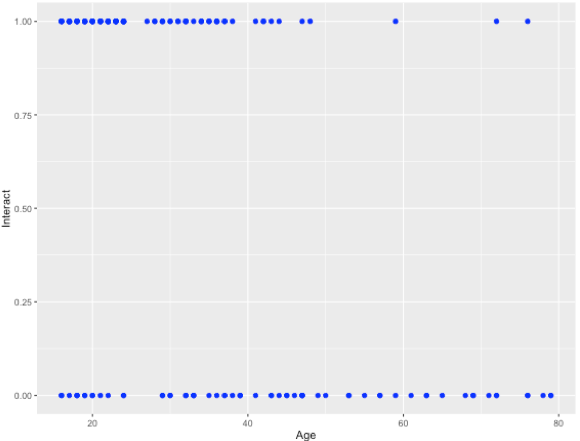
The age of the user is plotted on x-axis and user interaction with the app is plotted on the y-axis. “1” represents interactions whereas “0” represents non-interaction.
It appears in the graph above, that users under age 50 interact more frequently than those older than 50. This is represented by more dots leading up to 50 for “1” compared to “0”.
What is a Mosaic Plot?
A mosaic plot (also known as a Mekko chart) is a type of data visualization – an infographic, if you will – that helps you look at the relationship between two or more qualitative variables. The mosaic plot allows you to see how each variable relates to the overall picture and to one another.
Let’s group the users based on age and visualize the relationship with the help of a mosaic plot: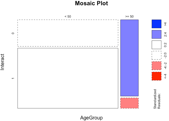
It is clear that there is a statistical significance for the group aged 50 or more as shown by the colors. It seems for users having age higher than or equal to 50 interact very less with the app compared to the global average for the app.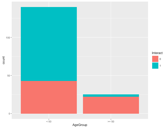
The bar chart shows that there is a skewed distribution of the data in regards to those younger than 50. This accounts for approximately 85% of the total users which is not desirable. We could also have looked at the distribution of age of the customers and create groups of customers based on a percentile approach to have a better distribution. But, that approach only takes age into account and ignores the need to create groups based on whether the user has interacted with the app.
To solve for this, we can use different techniques to arrive at a better classification. Decision trees is one such technique.
What are Decision Trees?
Decision trees, as the name suggests, uses a tree plot to map out possible consequences to visually display event outcomes. This helps to identify a strategy and ultimately reach a goal. The goal, or dependent variable, in this case, is to find out whether the users interact with the independent variable of age.
Decision trees have three main parts: a root node, leaf nodes and branches. The root node is the starting point of the tree, and both root and leaf nodes contain questions or criteria to be answered. Branches are arrows connecting nodes, showing the flow from question to answer. Each node typically has two or more nodes extending from it. The way a decision tree selects the best question at a particular node is based on the information gained from the answer.
Decision Tree Example
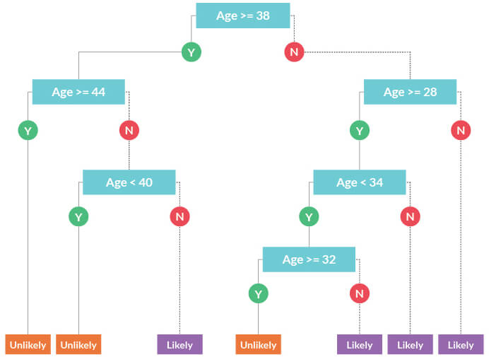
In the above example, the best question for the first node is whether the age of the user is greater than or equal to 38? This question was arrived after looking at the information gained from the answers for many such questions at varying users’ age. There is one leaf node for a “yes” response, and another node for “no.” We see such questions at each node based on whether the user is above or below a certain age.
Decision Tree Rules
Based on the above decision tree, we get certain rules based on which one could infer if a user is likely to interact with the app or not. Enumerated below are the rules:
Rule1 : Age < 38 -> Age < 28 = “Likely to interact”
Rule 2 : Age < 38 -> Age >= 28 -> Age >= 34 = “Likely to interact”
Rule 3 : Age < 38 -> Age >= 28 -> Age < 34 -> Age < 32 = “Likely to interact”
Rule 4 : Age < 38 -> Age >= 28 -> Age < 34 -> Age >= 32 = “Unlikely to interact”
Rule 5 : Age >= 38 -> Age >= 44 = “Unlikely to interact”
Rule 6 : Age >= 38 -> Age < 44 -> Age < 40 = “Unlikely to interact”
Rule 7 : Age >= 38 -> Age < 44 -> Age >= 40 = “Likely to interact”
From the above rules, it looks like we could classify the users in 3 age groups “< 28”, “>= 28 and < 44” and“>= 44”.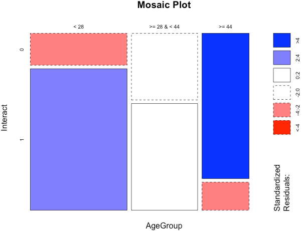
The mosaic plot indicates a statistical significance for age group “< 28” & “>= 44”. it seems users less than 28 years interact significantly more and users who are more than or equal to 44 years interact significantly less with the app compared to the global average. Users between the above age group interact as per the global average.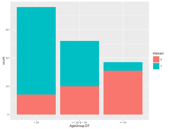
The chart above shows that the distribution of users among various age groups is not heavily skewed toward one user group compared to the earlier distribution. The above user segmentation is more useful and distributed compared to the earlier one. One could also create an additional categorical feature using the above classification to build a model that predicts whether a user would interact with the app.
With the help of Decision Trees, we have been able to convert a numerical variable into a categorical one and get a quick user segmentation by binning the numerical variable in groups. When using R to bin data this classification can, itself, be dynamic towards the desired goal, which in the example discussed was the identification of interacting users based on their age.
Source Code (R) and Dataset to reproduce the above article available here.
Jacob Joseph 
Heads Data Science.Expert in AI, Data & Analytics and awarded 40 under 40 Data Scientists in India.
Free Customer Engagement Guides
Join our newsletter for actionable tips and proven strategies to grow your business and engage your customers.