A brief primer on linear regression – Part II

In the first part, we had discussed that the main task for building a multiple linear regression model is to fit a straight line through a scatter plot of data points in multidimensional space, that best estimates the observed trend.
While building models to analyze the data, the foremost challenge is, the correct application of the techniques– how well analysts can apply the techniques to formulate appropriate statistical models to solve real problems.
Furthermore, before proceeding to analyze the data using multiple regression, part of the process encompasses to ensure that data you want to analyze, can actually be analyzed using multiple regression. Therefore, it is only appropriate to use multiple regression if you understand the key assumptions underlying regression analysis and check whether your data “passes” the required assumptions to give a valid result.
Usually, it’s plausible for one or more of the assumptions being violated, while analyzing real-world data. Even when the data fails certain assumptions, there is often a solution to overcome this. First, let’s look at the assumptions, and then learn how to check / validate the assumptions and also discuss about the proposed solutions for correcting these violations, if any.
We would be using IVs for independent variables and DV for dependent variable interchangeably while going through listing and validating assumptions, exploring data, building the model and interpreting the model output.
Assumptions of Regression:
Number of Cases/Sample Size
When conducting regression analysis, the cases-to-Independent Variables ratio should ideally be 20 cases for every independent variable in the model. For instance, the simplest case with two IVs – would require that n>40. However, for qualitative i.e. categorical variables with many levels of values, we might require more than ideal 20 cases for this variable to have sufficient data points for each level of categorical variable.
In this age of Big Data, we don’t need to worry about dealing with small samples. But, this assumption violation does result in generalizability issue of not being able to apply the model’s valuable insights and recommendations to other similar samples or situations.
Type of the Variables 
The dependent variable should be measured on a continuous scale (i.e. an interval or ratio variable). Examples include revision time (measured in hours), intelligence (measured using IQ score), exam performance (measured from 0 to 100), weight (measured in kg or pounds), and so on.
The two or more independent variables can be either continuous (i.e. an interval or ratio variable) or categorical (i.e. an ordinal or nominal variable).

• Examples of ordinal variables include Likert items – a 7-point scale from “strongly agree” to “strongly disagree” or other way of ranking categories – a 3-point scale to explain the liking of the product, from “Yes”, “No” and “May be”.
• Examples of nominal variables include gender (2 groups: male and female), ethnicity (3 groups: Caucasian, African-American and Hispanic), physical activity level (5 groups: sedentary, slightly active, moderately active, active, and extremely active), profession (5 groups: surgeon, doctor, nurse, dentist, therapist) and so forth.

Revisiting our weight–height example, we notice two of the independent variables to be continuous and one as categorical – exercise level with 3 levels.   Hence, for carrying out regression analysis, we need to create new variable(s) or recode the categorical variable – exercise level – into numerical values as the regression algorithm doesn’t work with non-numeric variables. Exercise level for each person can be recoded as (1=Sedentary, 2=Moderately Active, 3=Very Active) based on their lifestyle and attitude towards exercise.
Linearity
Multiple regression technique does not test whether the data is linear. Instead, it requires the existence of a linear relationship between – the dependent variable and each of the independent variables, and the dependent variable and the independent variables collectively (assessed from the model fit or from 3^rd scatterplot as shown below).The above plots help us to visually answer: Are the two variables linearly related? We infer that each of the IVs (height, calorie intake) in first 2 plots, plotted one at a time, with the dependent variable (weight) and even the last plot (effect of IVs collectively via Predicted values of DV) signifies linear relationship between the variables.
Normality
Multiple Regression Analysis requires that variables are normally distributed. In practice, the distribution of the variables, close to normal distribution is acceptable. There are various ways to check the normality assumption. Histogram is a quick way to check normality.

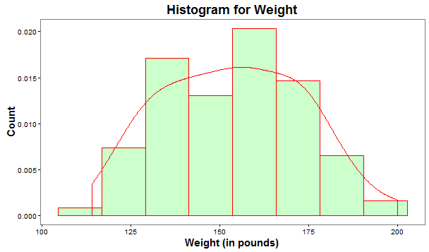
The above histogram plot includes a density curve that closely depicts the bell-shaped curve of normal distribution.

Absence of MultiCollinearity
Multicollinearity pertains to the relationship among IVs.  exists when the IVs are highly correlated with each other or when one IV is a combination of one or more of the other IVs.
For example, when we look into the pricing of house flat, both the variables – area in square feet and area in square cm or square inches doesn’t contribute much to the price prediction as these 2 variables give the same information, though in a different way and are highly correlated as evident from the conversion formula.

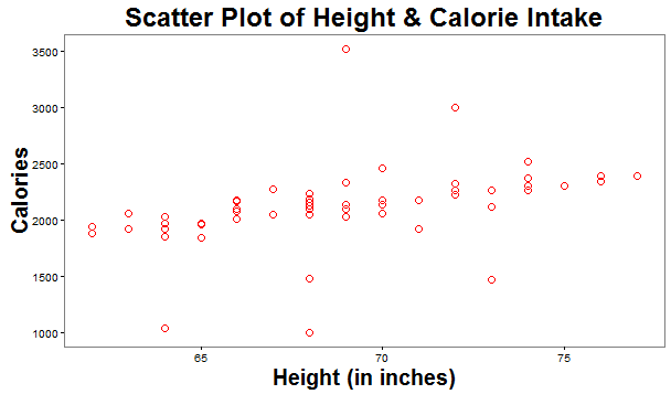As indicated in the above plot, height and calorie intake used for predicting weight reflects no discernible pattern i.e. the data demonstrates an absence of multicollinearity.

The other criteria that could be used to detect multicollinearity are Tolerance, Variance Inflation Factor (VIF), or Condition Index.
Absence of Significant Outliers among variables
There should be no significant outliers for both– among IVs and on DV. Outliers are points which lie outside the overall pattern of the data. The removal of these influential observations can cause the regression equation to change considerably and may improve correlation.
Potential outliers could be identified from the plots of each of the IVs and DV for weight – height example as below:The remedial measures for treating outliers could be:

• An outlier for a particular IV can be tackled either by deleting the entire observation, counting those extreme values as missing and then treat missing values, or retain the outlier by reducing the extremity by assigning a high score/value for that variable, but not too different from the remaining cluster of scores.
• Outliers on DV can be identified readily on residual plots since they are cases with very large positive or negative residuals (errors). In practice, standardized residual values greater than an absolute value of 3.3(i.e. above 3.3 or less than -3.3) are considered outliers.

Normality, Linearity, Homoscedasticity and Independence of Residuals
Residuals are the errors in prediction–the difference between observed and predicted DV scores.
These characteristics of Residuals illustrates the nature of the underlying relationship between the variables, which can be checked from residuals scatter-plots.
The residual scatter-plots allow you to check

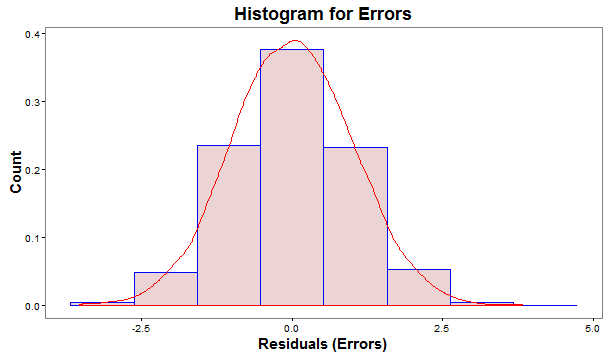
• Normality: The residuals should be normally distributed. Though, in practice, the distribution of errors, close to normal is acceptable.

The normality of errors could be gauged through:

  (i) Histogram of Errors– should be mound shaped around 0.

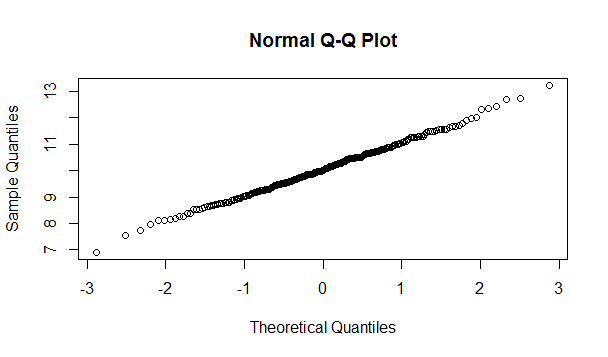
(ii) Normal Probability Plot (Q-Q plot)– is a scatter-plot created by plotting 2 sets of quantiles (often termed as “percentiles”) against one another. For example, the 0.3 (or 30%) quantile is the point at which 30% of the data fall below and 70% fall above that value. Q-Q plot help us to access if a dataset probably came from some theoretical distribution such as Normal, or other distribution.

(iii) Statistical tests like Correlation test, Wilks-Shapiro test etc

Linearity: The residuals plot should reflect a random scatter of points. A non-random pattern suggests that a linear model is inappropriate, and that data may require some transformation of the response or predictor variables or add a quadratic or higher term in the equation.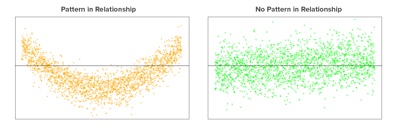 As seen in the above residuals plot – first one shows a pattern i.e. the relationship between IVs and DV is  not linear. Therefore, the results of the regression analysis would under-estimate the true relationship.

• Homoscedasticity: The scatter-plot is a good way to check whether homoscedasticity (i.e. the error terms along the regression are equal è constant variance across IV values) is given.

The homoscedasticity and heteroscedasticity plots of data reveals either no pattern or some pattern as shown below:

Heteroscedasticity i.e. non-constant variance of errors can lead to serious distortion in findings and weaken the analysis and increase the prediction errors. A non-linear transformation might fix this problem.

• Independence: The residuals should be independently distributed i.e. no correlation between consecutive errors. In other words, one of the error is independent of the value of another error(s).

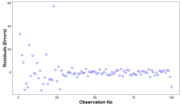
 A random pattern of Errors, as above indicates independence of errors.

Closing Thoughts:
It may happen that you get fascinated by the insights arising from your linear regression model, but you should force yourself to probe into the validity and conformance of the key assumptions underlying your regression model, so as to be able to apply it and get similar results from unseen or new data.
In the concluding part , we will learn how to build the regression model and interpret the model output to evaluate the quality of the model.