The first predictive model that an analyst encounters is Linear Regression. A linear regression line has an equation of the form,![]()
where X = explanatory variable, Y = dependent variable, a = intercept and b = coefficient.
In order to find the intercept and coefficients of a linear regression line, the above equation is generally solved by minimizing the squared of the errors (L2 norm loss function).

Why do we choose to minimize the squared errors? Can we not choose to minimize the errors with a power other than 2? We use the squared errors since we do not want to distinguish between positive or negative errors. Also, by using squared errors, we are able to get a closed form analytical solution in the form of Ordinary Least Squares (OLS). Since we square the errors, the model using L2 norm loss function is sensitive to those predicted points that are far away from actual/observed points and also less efficient for skewed error distributions as well as some symmetric error distributions that have fat tail.
Let’s take a simple example where we highlight the sensitivity of squared errors to outliers.
Table 1: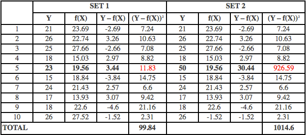
The above table contains the observed or the actual data for the dependent variable (Y), the predicted dependent variable (f(X)), the squared errors (Y – f(X))2. There are 2 sets of dependent observed variable and predicted variable. Whilst the first set of Y doesn’t contain any outliers, the second set contains the outlier. The value of ‘Y’ for observation no: 5 has changed from 23 to 50. It is quite clear that with the introduction of one outlier, there is drastic change in the sum of the squared errors from 100 to 1015. Hence, the coefficients of the predictive model will also see a dramatic shift so that the sum of squared errors are minimized or reduced.
Alternative Approach
An alternative approach to minimizing the errors is to minimize the absolute value of the error.
 In the above equation, we are trying to minimize the absolute errors instead of squared errors. The above argument seems familiar. A similar argument is made in favor of choosing Mean Absolute Deviation over Standard Deviation. One can deduce the fact from the above equation that Least Absolute Deviation (LAD) or L1 norm loss function is less likely to be affected by outliers compared to L2 norm loss function since it doesn’t square the deviation but takes its absolute value. Hence, the impact of large deviation of observed ‘y’ from predicted ‘y’ is less compared to L2 norm loss function. This is especially useful in case of outliers. The claim could be empirically verified from Table 1 where the sum of absolute errors increase from 31 to 58, which is considerably less, as compared to the increase in sum of squared errors.
Comparison
Let’s try and use an example to visualize the implication of using the error functions on a sample dataset.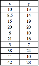
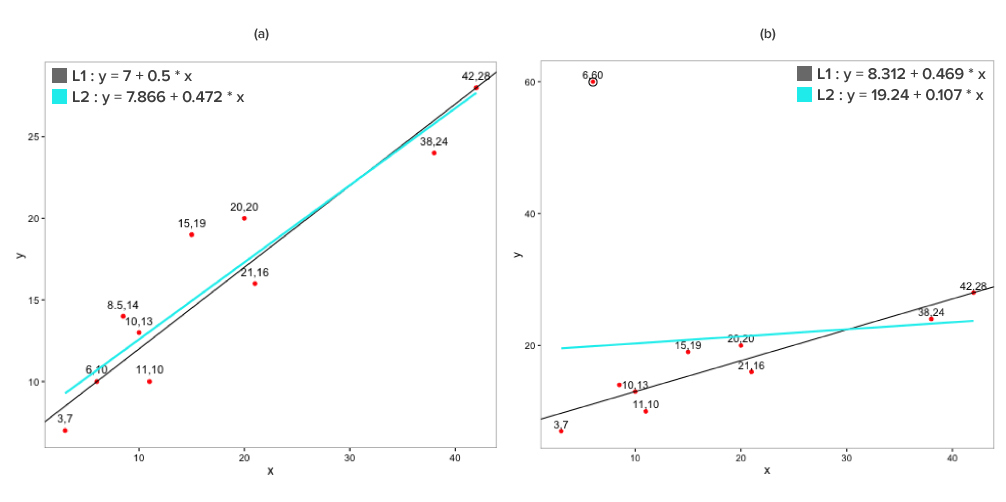
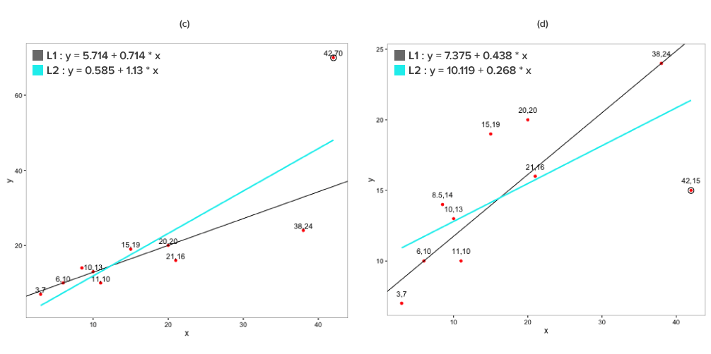 The above plots depict the linear relationship between x and y. The trend lines are linear regression lines using L1 norm loss function depicted in black and L2 norm loss function depicted in cyan. In plot (b), (c) and (d), one of the point in ‘y’ is changed, which changes the nature of such point to an outlier. The coefficients for the regression line are recalculated to assess the impact on the regression lines. It is quite evident from the trend lines that there is considerably less movement for regression line using L1 norm loss function as compared to L2 norm loss function due to the introduction of outliers.
Key Benefits of L1 norm over L2 norm
⇒ Outliers
As an analyst, you may choose to identify and treat the outliers by performing a univariate and/or bivariate analysis. Quite often the observations identified as outliers by the bivariate analysis may be different or a subset of the observations identified by univariate analysis. The complexity of identifying outliers is only bound to increase with multivariate analysis due to an increase in number of variables.
Instead of going through the painstakingly complex approach to identify and treat the outliers, one could instead choose to suppress the effect of outliers, which is where L1 norm loss function tends to be useful. Compared to L2 norm loss function, L1 norm loss function is more resistant to outliers and also robust to departures from the normality assumption for errors in regression.
⇒ Overfitting
Another useful scenario where L1 could be used, is to avoid Overfitting, which is common problem faced by analysts. In overfitting, a model fits the training or in-sample data but fails to generalize and hence, cannot be used as the model to predict on new data or out-of-sample data. While training the model on in-sample data, a model that overfits would try to fit the model perfectly to almost each and every observation of the target or dependent variable. As a result, the model would land up with large coefficients for few variables making the model sensitive to small changes in such variables.
In order to reduce or avoid overfitting, a slacking component in the form of Regularization is introduced. Regularization introduces a penalty, which grows in relation to the size of the coefficients and reduces its impact, thus making the model less sensitive to small changes in the variables. Though L2 norm is generally used for Regularization, L1 norm could be more beneficial.
L1 norm is also quite useful for sparse datasets. This is possible since L1 norm when used for Regularization tend to produce many coefficients with zero values or very small values with few large coefficients.
So why isn’t L1 norm used more often?
The primary disadvantage of L1 norm is that it is computationally more expensive than L2 norm and may not have a unique solution as compared to L2 norm loss function for solving regression type problems. The coefficients for L1 norm loss function are found iteratively compared to L2 norm loss function. Coefficients calculated using L2 norm loss function have a unique solution, courtesy its closed form analytical solution in the form of OLS, but, the problem of not having a unique solution may not be that acute when one is dealing with many independent variables or multidimensional space.
Closing Thoughts
In the real world, an analyst has to deal with the lurking and confounding dangers of outliers, non-normality of errors and overfitting especially in sparse datasets among others. Using L2 norm results in exposing the analyst to such risks. Hence, use of L1 norm could be quite beneficial as it is quite robust to fend off such risks to a large extent, thereby resulting in better and robust regression models.
Click here to reproduce the example comparing the impact of L1 and L2 norm loss function for fitting the regression line.
Do you agree with the benefit of using L1 norm over L2 norm? Please feel free to comment or write to me at [email protected]
Jacob Joseph 
Heads Data Science.Expert in AI, Data & Analytics and awarded 40 under 40 Data Scientists in India.
Free Customer Engagement Guides
Join our newsletter for actionable tips and proven strategies to grow your business and engage your customers.


