A brief primer on linear regression – Part III

In Part I, we learnt the basics of Linear Regression and in Part II, we have seen that testing the assumptions in simple and multiple regression before building a regression model is analogous to knowing the rules upfront before playing a fair game.
Building a regression model involves collecting predictor and response values for common samples, exploring data, cleaning and preparing data and then fitting a suitable mathematical relationship to the collected data to answer: Which factors matter the most? Which factors we can ignore?
In the linear regression model, the dependent variable is expressed as a linear function of two or more independent variables plus an error introduced to account for all other factors, as mentioned below:

Y = a + b₁x₁ + b₂x₂ + b₃x₃ + b₄x₄….+ b_nx_n + ϵ

Linear Regression Model Building
Prior to building any predictive model, the data exploration and preparation stage ensures that every variable is in the form as desired by model. The next step is to build a suitable model and then interpret the model output to assess whether the built model is a good fit for the given data.
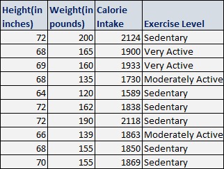
As a quick recap of our height – weight dataset, a sample of 10 rows of this dataset has been displayed below:

Let’s work on fitting a linear model to the above dataset by using height, calorie intake, and exercise level as predictors for predicting the response variable – weight of an individual and then derive valuable insights by interpreting the model output.
Interpreting the output
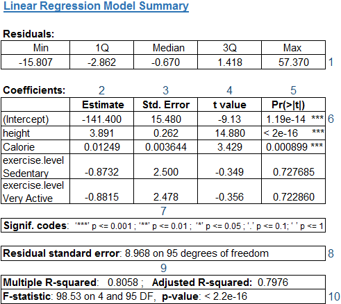
The model output for our height-weight example is displayed below:                                                                                           
This output includes a conventional table with parameter estimates and their standard errors, t-value, p-value, F-statistic, as well as the residual standard error and multiple R-squared.
Now we define and explain briefly each component – marked as #1 – #10 in the above model output.
#1 Residuals – are essentially the errors in prediction – for our example, the difference between the actual observed “Weight” values and the model’s predicted “Weight” values.
The Residuals section of the model output breaks down into 5 summary point measures, to help us assess whether the distribution of residuals is normal i.e. bell shaped curve across the mean value zero (0).
In our case, we see that the distribution of the residuals do not appear to be strongly normal as median is to the left of 0. That means the model predicts certain points that fall far away from the actual points.
Residuals can be thought of as similar to a dart board. A good model is the one which will hit the bull’s-eye some of the time. When it doesn’t hit the bull’s-eye, the miss should be close enough to the bull’s-eye than on the outer edges of the dart board.
#2 Estimated Coefficients – are the unknown constants that represent the intercept and slope terms in the linear model. The estimated coefficient is the value of slope calculated by the regression. 
As in the above table, the coefficient Estimate column contains two or more rows: the first one is the intercept and the rest rows are for each of the independent variable(s).

• The intercept is the base value for DV (weight) when all IVs (height, calorie, exercise level in our case) are zero. In this context, the intercept value is relatively meaningless since weight of 0 lbs is unlikely to occur for even an infant. Hence, we cannot draw any further interpretation from this coefficient.

• From the second row onwards there are slopes for each of the independent variables considered for building predictive model. In short, the size of the coefficient for each IV gives the size of the effect that variable has on the DV and the sign on the coefficient (positive or negative) gives the direction of the effect. For example, the effect height has in predicting weight of a person. The slope term of height indicates that for every 1 inch increase in the height of a person, the weight goes up by 3.891 pounds (lbs), holding all other IVs constant.

#3 & #8 Standard Error of the Coefficient Estimate & Residual Standard Error – are just the standard deviations of Coefficient Estimate and Residuals. The standard error of the estimate measures the dispersion (variability) of the coefficient, the amount it varies across cases and Residual standard error reflects the quality of a linear regression fit. Lower the standard error, the better it is, for accuracy of predictions. Therefore, you would expect to observe most of the actual values to cluster fairly closely to the regression line.
For example, to decide among the 2 datasets of 10 heights having same mean of 69 inches but different standard deviations (SD) – one with σ = 2.7 and the other one with σ = 6.3, we should select the dataset with σ = 2.7 to use height as one of predictor for creating predictive model.
In our example, the std error of the height variable is 0.262 which is far less than the height Coefficient – Estimate (3.891). Also, the actual weight can deviate from the true regression line by approximately 8.968 lbs, on an average.
#9 Multiple R-squared & Adjusted R-squared – The R-squared statistic (R²), also known as Coefficient of determination, is a metric used to evaluate how well the model fits the actual data.
R² corresponds with the proportion of the variance in the criterion variable which is accounted for, by the model.

R² always lies between 0 and 1. Hence, a number near 0 represents that a regression does not explain the variability in the response variable and a number close to 1 does explain the observed variance in the response variable.
R² tends to somewhat over-estimate the success of the model since it automatically and spuriously increases when extra explanatory variables are added to the model. Adj. R² corrects this value to provide a better estimate of the true population value by taking into account the number of variables and the number of observations that goes into building the model.

where p is the total number of variables in the model (excluding the constant – Intercept term), and n is the sample size.

Unlike R² – always increasing as more variables are included in the model, adjusted R² increases only if the new term improves the model more than what would be expected by chance. It decreases when a predictor improves the model by less than expected by chance. It is always lower than R². Furthermore, adj. R² is the preferred measure to evaluate the model fit as it adjusts for the number of variables considered.
While choosing between two models, it’s better to choose the one with higher adj. R². However, this higher value doesn’t necessarily indicate the accuracy of the predictions and the adequacy of the regression model.
In our case,  ~80% of the variance in the response variable (weight) is explained by the predictors (height and calorie intake). Intuitively also, by knowing these values – height, calorie intake – we would be able to predict the weight of an individual quite well, as also reflected in the obtained relatively strong R² value.
#4 – #7; #10 t – value of the Coefficient Estimate; Variable p – value, Significance Stars and Codes; F-statistic with Degrees of Freedom and p-value – are the terms used to assess the model fit and the significance of the model or its components through the statistical tests.
t – value of the Coefficient Estimate –
is a score to measure whether or not the regression coefficient for the variable is meaningful for the model i.e. the coefficient is significant and different from zero.
The t-statistic value is computed as:

In our example, the t-values of height, calorie intake are relatively far away from zero and are large relative to the standard error, which could indicate an existence of the relationship.
Variable p-value & Significance Stars and Codes –
p-value indicates a probability that the variable is NOT relevant i.e. Pr(>(|t|) acronym in the model output. A small p-value indicates that it is unlikely that a relationship between a predictor (say, height) and response (weight) variables exists due to chance. Generally, a p-value of 5% or less is considered as cut-off point.
In our example, the p-values for height and calorie intake are very close to zero (indicated by ‘***’ in the table), suggesting that it is likely that significant relationship exists between height, calorie intake and weight of the people – with the obtained coefficient estimates – different from zero.
F-statistic, Degree of Freedom and Resulting p-value –
are the metrics to evaluate the overall model fit of the data. F-statistic is a good indicator to assess whether there is a relationship between the dependent and independent variables. The further F-statistic is from 1, the higher the likelihood of the existence of relationship between dependent and independent variables.
To explain Degrees of Freedom, let’s consider a scenario where we know 9 of the data points and the mean of 10 data points. We don’t have freedom to choose the actual value of 10^th observation, as we can easily calculate the same by (mean * 10 – Sum of all 9 observations). This results in one data point going into estimating this actual value of 10^th data point, giving us choice of 9 degrees of freedom (d.f.) for these 9 known points.
In our example, the F-statistic is 98.53 which is much larger than 1 given in the 100 observations. The degrees of freedom are 4 (the number of variables used in the model (5 – including Intercept) – 1) and 95 (the number of observations included in the dataset (100) – the number of variables used in the model (5)). Also, the p-value is low and close to 0. Hence, a large value of F and small p-value indicates the overall significance of the model.
Closing Thoughts

It is often trickier to spot a bad model rather than identifying and selecting a good model.

Multiple regression analysis is not only the most widely used tool but also the most abused one. Furthermore, the sensible use of linear regression requires one to check for any errors in variables, treat outliers and any missing values, validate the underlying assumptions for any violation(s); determine the goodness of fit  and accuracy of the model through statistical tests; deal with potential problems that may occur in the model and the difficulties involved in rigorously evaluating the quality and robustness of the model fit. Linear regression is important because it is the basic model used by many analysts to compare with other complex models to generate data insights.