A brief primer on linear regression – Part I

Prediction has always been a curious topic in life due to a key attribute – the extreme human desire to know what is coming next.
Let’s ponder over our thoughts to answer a simple question – “Where is prediction most relevant in your life today?”
Predictions are central to every aspect of our life, whether we realize it or not. During school days, it was predicting what we would love to do in the future to choose a career path, checking the weather today to determine how should I dress, evaluating inventory numbers for the next day, to less important predictions made daily during our interactions with other people – like doing time management and getting into classes for a student, to dining, socializing, etc.
So, what’s a prediction?
A prediction or forecast, is a statement about the future. It’s a guess, sometimes based on knowledge or experience, but not always.
Now, let’s consider a popular and common use case of the speed of an object to understand how predictions play an important role in our real world; in shaping our lives in ways and instances that we aren’t aware of at first, and thereby help us to make informed decisions.
Have you ever thought of or answered day-to-day questions like –

• How fast vehicles such as cars and trains can go and how their speeds are calculated?
• When a police officer gives someone a speeding ticket, how does she know for sure if the person was speeding?

These questions force us to recollect our old learnings and refresh the concept of the physical system – the speed of an object is the magnitude of its velocity (the rate of change of its position) i.e. the speed of a certain object is calculated by dividing the distance travelled by the time taken to travel that distance.
At first glance, the above equation states that speed is a function of two quantities – distance and time. But, it really is a simple linear relationship called the rate formula because at least one of the 3 variables will always be a constant depending on the problem on hand.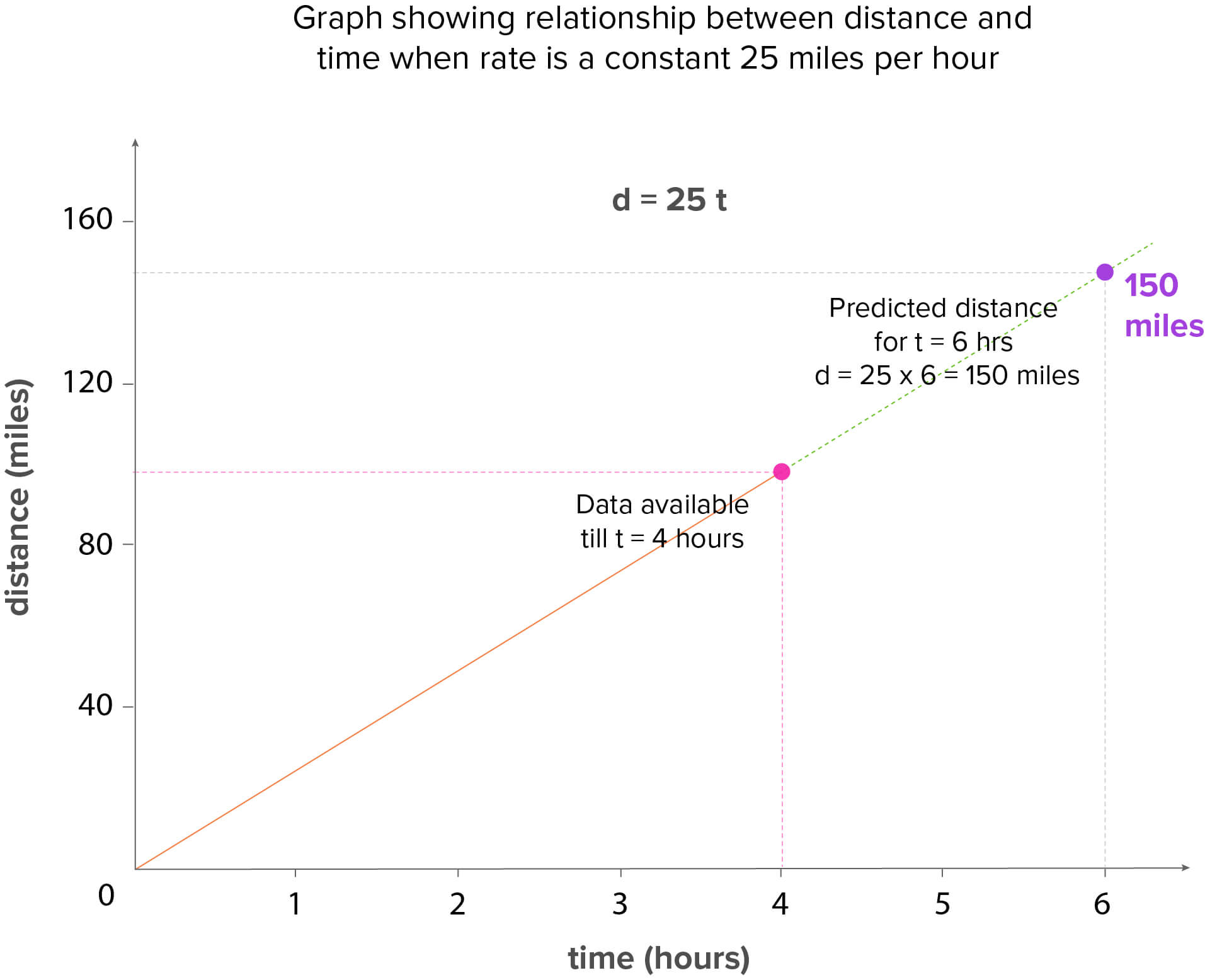The perfect linear relationship, as prevalent in the physical systems due to their inherent nature, are termed as Deterministic (or functional) relationships – comprising of an equation, that exactly describes the relationship between the two variables. Other examples could be

• Fahrenheit degree and Celsius degree (Fahr = 9/5 Cels + 32),
• Circumference (Circumference = pi x diameter) and
• Exchange rate conversion formula (new currency = (exchange rate) x (your currency))

Generally, we do come across scenarios depicting Statistical relationships – where the relationship between the two variables is not perfect, but there could be negative or positive relationship between the variables. Some examples could be

• Height and weight – as height increases, weight might increase but not perfectly
• Driving speed and gas mileage – as driving speed increases, gas mileage is expected to decrease, but not perfectly

These relationships, not of perfect kind nature, when graphed, gives a scatter plot of points, as seen from the plot of height-weight information of 30 adults as below:The above scatter plot reflects the relationship between height and weight as linear, depicting a positive increase in weight with height. We can thus fit a straight line to this data which would provide the best estimate of the observed trend.
The data points in the above scatter plot could be summarized in many ways as shown by various lines in the below plot: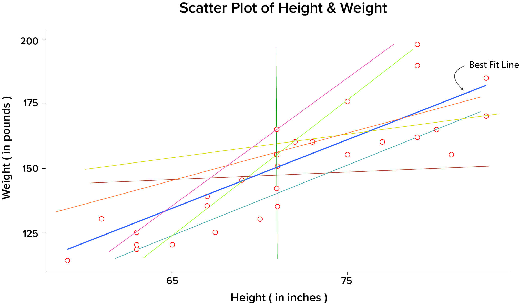Now the question arises – What is the best fit line that summarizes the relationship between height-weight, amongst all possible lines?
The best fit line is the one in blue color, and termed as regression line, which is actually the plot of the predicted score on y, for each possible value of x.
But, the next question comes – how to arrive at this best line?
The best line fitting the given data is obtained by “minimizing the residual variation” as below

The closer the regression line comes to all the data points on the scatter plot, the better it is. This means that the minimum variation of points around the line results into low prediction error.
The best fit straight line to summarize the data, as described above, could be obtained by using a prediction method such as Simple Regression.
What is Simple Linear Regression?
Simple Linear Regression is a statistical technique that allows us to summarize and study relationships between two continuous i.e. numeric variables:

• The variable we are predicting is called the criterion or response or dependent variable, and
• The variable we are basing our predictions on is called the predictor or explanatory or independent

Simple linear regression gets its adjective ‘simple’, because it concerns the study of only one predictor variable.
For example, the height-weight information of 100 randomly selected people, aged between 20 and 60, can be quantified in terms of the equation or model, considering the response variable as weight and one predictor variable as height. Here, the inherent assumption, though quite unrealistic, is that “weight” can be measured by a single attribute – height. The model to fit this data could be written as
Weight (continuous)  ̴  Height (continuous)
In contrast, multiple linear regression, gets its adjective ‘multiple’, because it concerns the study of two or more predictor variables.
Extending our classic example of height-weight, we include other predictor variables, say, calorie intake, exercise level that would affect the person’s weight. The model to fit this data could be written as
Weight (continuous)  ̴  Height (continuous) + Calorie Intake (continuous) + Exercise Level (categorical)
A sample dataset of 10 rows pertaining to height-weight example along with other factors affecting the prediction is displayed below: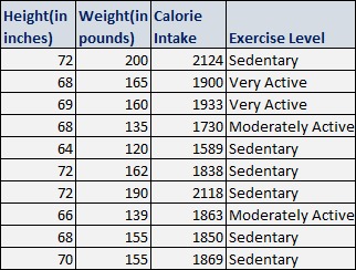

Both height and calorie intake individually are linearly related to weight as seen below in their scatter plots.However, both height and calorie intake together may affect the weight of an individual linearly in a multi-dimensional cloud of data points, but not in the same manner as they affect alone, in the above scatter plots.
The general mathematical model for representing the linear relationships (termed as regression equations) can be written as:Here, for simple regression – b, the slope of the linear equation indicates the strength of impact of the variable, and a, the intercept of the line. And for multiple regression – b_i (i =1, 2, …,n), are the slopes or regression coefficients, indicates the strength of impact of the predictors, and a, is the intercept of the line.
The regression coefficient estimates the change in the response variable Y per unit increase in one of the x_i (i =1, 2, …,n) when all other predictors are held constant i.e. for our height-weight example, if x₁ differed by one unit, and  both x₂  and x₃ are held constant, Y will differ by b₁ units, on an average.
The intercept or Y-intercept of the line, is the value you would predict for Y if all predictors are 0 i.e. when all x_i = 0 (i =1, 2, …,n). In some cases, the Y-intercept really has no meaningful interpretation, but it just helps to anchor the regression line in the right place.
Conclusion
In this part, we introduced simple linear regression model with one predictor variable and then extended it to the multiple linear regression model with at least two predictors.
A sound understanding of regression analysis, and modeling provides a solid foundation for analysts to gain deeper understanding of virtually every statistical and machine learning technique. Although regression analysis is not the fanciest learning technique, it is a dominant and widely used statistical technique to establish a relationship model between two or more variables.
In the ensuing part, we will delve into the steps and methodology to develop multiple linear regression model.