Learn how you can Unlock Limitless Customer Lifetime Value with CleverTap’s All-in-One Customer Engagement Platform.
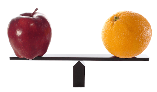
How often have you come across the idiom “Comparing apples and oranges”. It is a great analogy to articulate that two things can’t be compared due to the fundamental difference between them. As an analyst, you deal with such difference and make sense of it on a daily basis.
Let’s take an example and understand some ways to compare apples and oranges.
We will attempt to understand ways to compare apples and oranges by transforming the data and its key metrics. Please read this article, if you need to compare relationship of different types of variables visually.
We will start with numerical variables. Consider you have the below dataset and you need to compare the variables: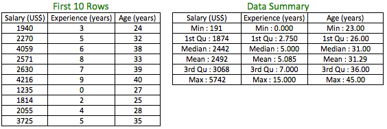
The first thing to hit you is all the above 3 variables in the dataset are different. But, the job of an analyst is to bring order in chaos by making sense of data. Some of the questions that may come to your mind:
a) Which variables vary the most?
b) How related are the variables?
c) Can I use these variables in my predictive model directly?
Let’s take the above questions one by one and attempt to answer them.
We need to compare the variation between variables to answer the above question. But, first we need to know how the variables vary or the measure of their dispersion. Variance is a popular measure of dispersion or variation.
^{2}}{\mathrm{N}}")
Steps involved in calculating the Variance:
Step 1) Calculate the mean (average) of the variable,
Step 2) Subtract mean from each of the observation and square it,
Step 3) Sum up the values obtained from Step 2,
Step 4) Divide the value obtained in Step 3 by the number of observations.
The above steps attempt to capture the average deviation of each observation of the variable from the mean. As a result of step 2 and step 3, a positive or a negative deviation from the mean only increases the variance. The variables in the example have their own unit measurements; Salary in dollars, Experience in years and Age in years. The unit of measurement for Variance is square of its respective unit (see Step 2 above). Standard Deviation is obtained by taking the square root of the Variance. This results in the measurement unit of Standard Deviation to be same as the original unit of measurement of the variable.
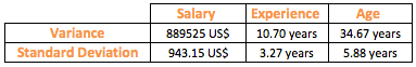
The above table gives us the variance and the standard deviation for the 3 variables. Since we have the measure of variation for all 3 variables, can we compare the variation among them? The answer is an emphatic “NO” since the variables are not measured on the same scale or unit.
Can we make some modification to the standard deviation to make it comparable? What if we make standard deviation unitless? This is where mean comes to our rescue. Mean is measured in the same unit as that of the Standard Deviation. Dividing standard deviation by mean achieves our objective and the result is known as Coefficient of variation.
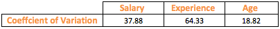
From the above table, it seems that Experience shows more variation than the other variables. Coefficient of variation has enabled us to compare the degree of variation in the variables even though they have drastically different means and scale.
Analyzing relationship between variables requires key metrics as well as visualization either to support the metrics or understand the variables or its relationship better. One metric, which is the most common and popular to understand relationship between numerical variables, is Correlation. To understand correlation, let’s look at covariance first:
The formula is essentially a variation of the variance formula with the first 2 steps of calculating variance replaced with the following 2 steps:
Step 1: Calculate the mean of the 2 variables
Step 2: Subtract respective means from the observations of the respective variables and multiply the results obtained
Rest of the steps remains the same as that of Variance. In this case, the steps attempt to capture the average deviation of 2 variables from their respective means simultaneously. Covariance can either be positive, if the variables move together or negative, if they move in the opposite direction (see step 2).

Covariance suffers from the same problem that we faced with Variance due to the units attached to it. So the unit for covariance between Salary and Age will be dollars x years. We need to get rid of the units and standardize covariance to enable comparison. If you have noticed, the unit of the covariance is a multiplication of the units of the 2 variables. What if we divide the covariance by the respective standard deviations of the 2 variables? Since standard deviation is measured in the unit of the variable, multiplying the standard deviation of the 2 variables will yield the same measurement unit as that of covariance, thereby resulting in unitless measure, when we divide both.
Correlation coefficient is bounded with lower bound of -1 and upper bound of +1. The closer the metric is to both the bounds, higher is the movement of the variables together or against each other. If the correlation coefficient is closer to -1 (negatively correlated), the variables move against each i.e. if one moves up the other falls. Likewise, if the correlation coefficient is closer to 1 (positively correlated), the variables move together i.e. if one moves up, the other follow.

As per the table, there seems to be a strong positive relationship among all the variables with the highest between Salary and Experience, since the correlation coefficient is positive for all and close to +1.
When you compare variables, you look at relative metrics rather than absolute metrics. You won’t be looking at coefficient of variation of Salary in insolation but compare it with the other 2 variables. The first 2 questions attempted to compare the individual metric. But, what if the goal was to compare the observations of the entire dataset rather than an individual metric of the variables. Building predictive models requires the entire dataset as the input.
Can you use the variables in the dataset as the input directly, especially if you use machine learning algorithms? Do you want your algorithms to give importance to variables just because their value is relatively high than other variables? In our example, Salary is on the highest scale. So, if we give all the variables in our dataset as an input to K-means, a popular machine learning algorithm, the algorithm will tend to give more importance to ‘Salary’ and the resultant clusters will be formed, probably segmenting just Salary and not the other variables in conjunction. This is because the algorithm just sees the values of the variables. So if K-means clusters the observations based on the numeric distance between observations, it is logical that Salary gets a higher weight in determining how the observations get clustered since its value is much higher than the other 2 variables.
What’s the way out? We have looked at standardizing individual metrics till now and not the entire data. Let’s look at a method to standardize the entire variable data using z-score.
In the above formula, we are subtracting each observation from its mean and dividing the result by the standard deviation. If you look at the formula closely, the resultant z-score is unitless as the units get canceled out due to the division.
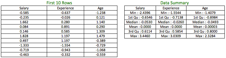
The table on the left shows the z-scores for the first 10 rows of the variables and the table to the right shows the data summary of the variables, post transformation.
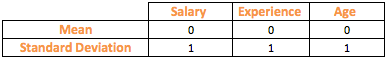
As seen from the above table, z-scores for the variables have transformed their mean to zero and standard deviation to 1.
There are situations where you require standardization, especially in machine learning techniques like PCA, K-means, etc but, at the same time, you might be required to transform the data into a particular range like in image processing, where pixel intensities have to be normalized to fit within a certain range (i.e., 0 to 255 for the RGB color range). Also, neural network algorithms may use data that are on a 0-1 scale in a way to avoid bias. This bias may arise due to the observations that are at the extreme end of the range or are outliers. To avoid such issues, a transformation technique, which bounds the data within a range, is required. This is can be achieved with Normalization.
Just like standardization, normalized data too is unitless. Let’s see what does our original dataset look like after normalization.
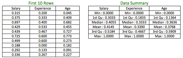
The table on the left shows the normalized scores for the first 10 rows of the variables and the table to the right shows the data summary of the variables, post transformation. All the variables are bounded between 0 and 1.
So how would you select between Standardization and Normalization? Depending on the objective of the technique, the method has to be selected. For techniques like PCA or K-means, you would like to retain the unbounded nature and the variation in the data while at the same time make the data unitless and relatively on same scale (range of transformed variable values). In such a case, Standardization is your best bet. There are times when you don’t want your data to be unbounded like in the case of Standardization so that your technique does not give a bias to observations, which are towards the higher/lower side of the range (potential outliers). Normalization reduces the impact of outliers as the range of the data is strictly between 0 and 1.
Comparing different variables should first involve identification of the purpose of such comparison depending on which the appropriate technique to transform the variables or the key metric should be selected. With the help of an example, we looked at coefficient of variation, correlation, standardization and normalization as some of the ways to compare and use different numerical variables for analysis and build predictive models on.
In the ensuing part, we will discuss how to compare categorical variables.